Author: Andrew Dupuis

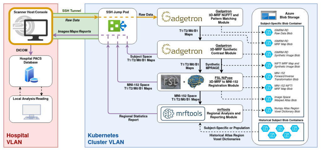
This post walks through running an mrftools offline MR Fingerprinting (MRF) reconstruction end-to-end, entirely in Docker, using two repositories — python-ismrmrd-server (reconstruction server) and python-ismrmrd-client (data converter + streaming client) — plus a sample raw-data file provided separately (it’s not in either repo).

The workflow is the same for every mrftools recon — prostate, abdomen, brain, etc. Only four things change between them. This guide uses the prostate case as the worked example and then shows exactly what to swap for others.

• Worked example dataset: meas_MID00758_FID33521_mrftools_prostate_yong.dat
• Worked example recon: mrftools_prostate_threaded (threaded, slice-by-slice)

The pipeline:

 .dat  ──(siemens_to_ismrmrd)──►  .h5 (MRD raw)  ──(client → server recon)──►  output .h5 (T1/T2/M0 maps)  ──(h5tomat)──►  .mat

This was run and verified end-to-end; the prostate maps below match the project’s known-good reference for this case to within floating-point rounding (correlation ≈ 0.99999999).

---

What you need

You have two git repositories and a sample data file. Put the repos somewhere together and keep your data somewhere of your choosing:

~/mrf/                          # any working directory
├── python-ismrmrd-server/      # repo 1 — the recon server
└── python-ismrmrd-client/      # repo 2 — the converter + client

~/mrf-data/                     # any data directory (provided separately)
└── meas_MID00758_FID33521_mrftools_prostate_yong.dat

To keep the commands copy-pasteable, set two environment variables — your repo root and your data directory:

export REPOS=~/mrf            # holds python-ismrmrd-server and python-ismrmrd-client
export DATA=~/mrf-data        # holds the .dat, and will receive the .h5 outputs

Raw data is always mounted in, never built into an image. The client’s .dockerignore deliberately excludes data, so you pass your .dat/.h5 files into the containers at run time with -v "$DATA":/data. Nothing about your data needs to live inside either repo.

---

Prerequisites

• Docker (with docker compose v2). Verified with Docker 29.5.
• NVIDIA GPU + nvidia-container-toolkit strongly recommended. The recon uses a NUFFT on the GPU (torch + torchkbnufft). It falls back to CPU automatically, but a full multi-slice case takes seconds on GPU vs. many minutes on CPU.
• ~10 GB free RAM and ~5 GB disk in $DATA for the intermediate MRD .h5 (a typical input .dat is ~2 GB; the converted MRD is similar).
• The server image is large (~29 GB — it’s based on the NVIDIA PyTorch container).

---

Step 1 — Build the client image (converter + streaming client)

The client image bundles siemens_to_ismrmrd (Siemens .dat → MRD .h5) and the streaming client.py. It’s the same image for every recon.

docker build -t mrd-client "$REPOS/python-ismrmrd-client"

This produces a small (~650 MB) image named mrd-client.

---

Step 2 — Build the reconstruction server image

The server image contains the mrftools reconstruction modules and PyTorch. One image serves all recon configs — you select which one at run time in Step 5.

cd "$REPOS/python-ismrmrd-server"
docker compose build

This builds the image tagged python-ismrmrd-server-mrf-recon from docker/Dockerfile, using the build settings in docker-compose.yml. The build is long the first time (it compiles ISMRMRD + siemens_to_ismrmrd and pulls the NVIDIA PyTorch base).

GPU note: the provided docker-compose.yml does not request a GPU. To run the recon on the GPU, start the server with the manual docker run command in Step 4, Option B (which adds --gpus all). docker compose up works too but runs on CPU.

---

Step 3 — Convert the Siemens .dat to MRD .h5

⚠️ The custom parameter map is required. mrftools MRF sequences store the image matrix size in vendor-specific header fields. With the default siemens_to_ismrmrd stylesheet, reconSpace.matrixSize.x comes out as 0 and the recon crashes with ZeroDivisionError: float division by zero (the NUFFT grid size becomes 0×0). You must pass the mrftools parameter map (-m) and stylesheet (-x), which are baked into the client image at /opt/code/python-ismrmrd-client/.

Run the converter inside the client container. Your data directory is mounted at /data, so the input .dat and the output .h5 both live in $DATA:

docker run --rm \
  -v "$DATA":/data \
  mrd-client \
  siemens_to_ismrmrd \
    -f /data/meas_MID00758_FID33521_mrftools_prostate_yong.dat \
    -z 2 \
    --skipSyncData \
    -m /opt/code/python-ismrmrd-client/mrftools_parameter_map.xml \
    -x /opt/code/python-ismrmrd-client/mrftools_brain_prod.xsl \
    -o /data/meas_758.h5

Flags:

Flag	Meaning
-f	input Siemens .dat file
-z 2	convert measurement 2 of this multi-RAID file (measurement 1 is calibration/AdjCoilSens; the MRF acquisition is the last measurement)
--skipSyncData	skip PMU/waveform (ECG/resp) data — required for Siemens XA60 data to avoid a PMU-parsing bug in siemens_to_ismrmrd v1.2.6
-m … mrftools_parameter_map.xml	custom Siemens parameter map (populates the matrix size)
-x … mrftools_brain_prod.xsl	custom stylesheet matching that parameter map (despite the “brain” name, this is the shared mrftools stylesheet)
-o	output MRD .h5

You’ll see wrote scan : N progress, then warnings about “additional bytes at the end of file” — these are benign for this file.

Sanity-check the header (the recon needs a non-zero matrix size):

docker run --rm -v "$DATA":/data mrd-client python -c "
import h5py, ismrmrd
hdr = ismrmrd.xsd.CreateFromDocument(h5py.File('/data/meas_758.h5','r')['dataset/xml'][0])
e = hdr.encoding[0]
print('encodedSpace:', e.encodedSpace.matrixSize.x, e.encodedSpace.matrixSize.y, e.encodedSpace.matrixSize.z)
print('reconSpace: ', e.reconSpace.matrixSize.x,  e.reconSpace.matrixSize.y,  e.reconSpace.matrixSize.z)
"

Expected (good) output for the prostate case:

encodedSpace: 256 256 1
reconSpace:  256 512 1

If reconSpace shows 0 0 1, the custom map/stylesheet were not applied — re-check Step 3.

---

Step 4 — Start the reconstruction server

The server listens on TCP port 9002. On first run it auto-downloads the MRF dictionary and spiral trajectories for the requested recon from Azure and caches them in Docker volumes (dictionary-data, b1-data, debug-data), so subsequent runs are fast. The Azure connection string is baked into the image. The same server handles every recon config; you choose the config on the client side in Step 5.

Behavior is configured through environment variables in python-ismrmrd-server/.env (coil count, T1/T2 ranges, B1 correction, iteration count, etc.).

Option A — docker compose up (simplest, CPU)

cd "$REPOS/python-ismrmrd-server"
docker compose up

Because network_mode: host is set, port 9002 is exposed directly on your host. This runs the recon on CPU (the compose file requests no GPU).

Option B — manual docker run (recommended — enables GPU)

In a separate terminal, start the server with GPU access and the cache volumes mounted. (Override the entrypoint so we can pass -v for verbose logging.)

cd "$REPOS/python-ismrmrd-server"

docker run -d --name mrf-server \
  --gpus all \
  --network host \
  --env-file .env \
  -v python-ismrmrd-server_dictionary-data:/usr/share/dictionary-data \
  -v python-ismrmrd-server_b1-data:/usr/share/b1-data \
  -v python-ismrmrd-server_debug-data:/usr/share/debug \
  --entrypoint python3 \
  python-ismrmrd-server-mrf-recon \
  /opt/code/python-ismrmrd-server/main.py -v -H=0.0.0.0 -p=9002

Confirm it is listening:

docker logs mrf-server --tail 5
# ... Starting server and listening for data at 0.0.0.0:9002
# ... Serving...

The volume names python-ismrmrd-server_* are the ones docker compose creates. If you never ran compose, Docker will create fresh empty volumes here and the first recon will download the dictionary from Azure (~170 MB for prostate).

---

Step 5 — Run the reconstruction (client → server)

With the server running, stream the converted MRD file to it. The -c <config> flag selects the recon module by name (the server imports the matching <config>.py). For the prostate example that is mrftools_prostate_threaded.

docker run --rm \
  --network host \
  -v "$DATA":/data \
  mrd-client \
  python client.py \
    -a localhost -p 9002 \
    -c mrftools_prostate_threaded \
    -o /data/output_758.h5 \
    /data/meas_758.h5

Flags: -a/-p server address/port, -c server-side config (recon module) name, -o output file, last positional arg is the input MRD file.

The client streams ~13,800 acquisitions; the server reconstructs slice-by-slice and streams images back. On a successful run the client prints a summary like:

Sent 13824 acquisitions  |  Received     0 acquisitions
Sent     0 images        |  Received    24 images
Session complete

24 images = 8 slices × 3 parameter maps (T1, T2, M0). (Image and slice counts vary by dataset/recon.) Watch the server side with docker logs -f mrf-server to see per-slice progress. The result is $DATA/output_758.h5.

---

Step 6 — Convert the output to MATLAB .mat (optional)

h5tomat.py (shipped in the client repo) repackages the parameter maps into a MATLAB-friendly .mat:

docker run --rm \
  -v "$DATA":/data \
  mrd-client \
  python h5tomat.py /data/output_758.h5

Produces $DATA/output_758.mat with datasets t1big_all, t2big_all, m0big_all (each [n_slices, rows, cols] float64), loadable in MATLAB via load('output_758.mat').

If your mrd-client image predates h5tomat.py being added to the Dockerfile, mount the repo’s copy in: -v "$REPOS/python-ismrmrd-client/h5tomat.py":/opt/code/python-ismrmrd-client/h5tomat.py:ro

---

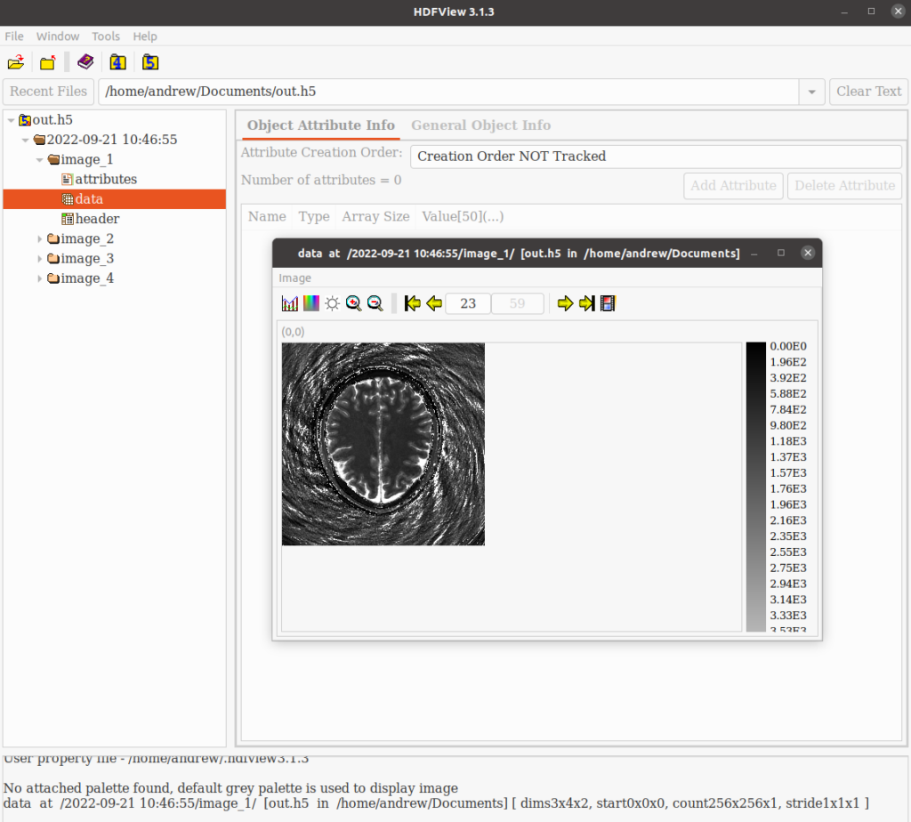
Step 7 — View the results (on the host, not Docker)

The viewer scripts in the client repo use a GUI and run on the host. They need matplotlib, numpy, h5py (and scipy for .mat):

cd "$REPOS/python-ismrmrd-client"
python view_images.py "$DATA/output_758.h5"     # MRD image viewer
python view_maps.py   "$DATA/output_758.mat"    # parameter-map viewer

view_images.py controls: ←/→ timepoint, ↑/↓ slice, +/- channel, r color range, q quit. The T1/T2/M0 montage near the top of this post was produced from output_758.h5 this way.

---

Adapting to other mrftools reconstructions

The steps above are identical for every mrftools recon. To run a different case, change only these four things:

What changes	Where	Prostate example	How to find it
1. Input dataset	Step 3 -f	..._prostate_yong.dat	the .dat for your anatomy (e.g. ..._abdomen_...dat)
2. Measurement number	Step 3 -z N	-z 2	the last measurement in the multi-RAID file (try -z 1, -z 2, … or -Z to dump all). Measurement 1 is usually calibration.
3. Recon config name	Step 5 -c <config>	mrftools_prostate_threaded	the server-side module name for that recon (matches a <config>.py in the server repo)
4. Trajectory / FOV / dictionary	automatic	FOV 400, 256², spiral	nothing to do — the recon reads FOV/matrix from the MRD header and picks the matching trajectory + dictionary itself

Everything else — the custom -m/-x conversion maps, --skipSyncData, the server launch, the dictionary/trajectory auto-download and caching, h5tomat.py, and the viewers — is shared.

The custom stylesheet is named mrftools_brain_prod.xsl for historical reasons but is the shared mrftools parameter stylesheet — use it for prostate, abdomen, brain, etc.

---

Adding a new reconstruction config to the server

A “config” is nothing more than a Python module in python-ismrmrd-server/ that exposes a process() function. When the client connects with -c <name>, the server runs importlib.import_module("<name>") and calls its process(). So adding a recon = dropping in a <name>.py file in the server repo. No registration, no edits to server.py.

1. Write the module

Create python-ismrmrd-server/myrecon.py. The minimal contract is a process() function that reads from the connection and sends images back. This example does a basic Cartesian FFT recon and is a good starting template:

import ismrmrd
import logging
import numpy as np
import numpy.fft as fft
import mrdhelper


def process(connection, config, metadata):
    logging.info("myrecon: starting (config='%s')", config)

    # Collect raw k-space acquisitions; ignore other message types.
    acqs = [item for item in connection if isinstance(item, ismrmrd.Acquisition)]
    if not acqs:
        connection.send_close()
        return
    logging.info("myrecon: received %d acquisitions", len(acqs))

    # Sort readouts into a Cartesian grid: [coils, ky, kx].
    ncoils = acqs[0].data.shape[0]
    nx = max(acq.data.shape[1] for acq in acqs)
    ny = max(acq.idx.kspace_encode_step_1 for acq in acqs) + 1
    kspace = np.zeros((ncoils, ny, nx), dtype=np.complex64)
    for acq in acqs:
        ky = acq.idx.kspace_encode_step_1
        kspace[:, ky, :acq.data.shape[1]] = acq.data

    # 2D inverse FFT + sum-of-squares coil combine, normalize to int16.
    img = fft.fftshift(fft.ifft2(fft.ifftshift(kspace, axes=(1, 2)), axes=(1, 2)), axes=(1, 2))
    img = np.sqrt(np.sum(np.abs(img) ** 2, axis=0))
    img = (img * (32767.0 / img.max())).astype(np.int16)

    # Wrap as an MRD image (copies orientation from the acquisition) and send it back.
    mrd_img = ismrmrd.Image.from_array(img, acquisition=acqs[0])
    mrd_img.image_index = 0
    connection.send_image(mrd_img)
    connection.send_close()

Notes:

• The function must be named process and accept (connection, config, metadata). The server first tries to call it with an extra version= keyword and silently falls back to this 3-argument form, so the signature above is fine.
• connection is an iterator of incoming MRD messages — filter for the types you want (ismrmrd.Acquisition for raw k-space, ismrmrd.Image for image input).
• Send results with connection.send_image(...) and finish with connection.send_close().
• invertcontrast.py and mrftools_prostate_threaded.py in the server repo are fuller references to copy from.

2. Test it without rebuilding (fast dev loop)

The server calls importlib.reload() on each connection, so if you mount the server repo as a volume, you can edit the module and re-run the client without restarting the server or rebuilding the image.

Start a dev server with the repo bind-mounted over the baked-in code:

cd "$REPOS/python-ismrmrd-server"

docker run -d --name mrf-server-dev \
  --gpus all --network host --env-file .env \
  -v "$(pwd)":/opt/code/python-ismrmrd-server \
  -v python-ismrmrd-server_dictionary-data:/usr/share/dictionary-data \
  --entrypoint python3 \
  python-ismrmrd-server-mrf-recon \
  /opt/code/python-ismrmrd-server/main.py -v -H=0.0.0.0 -p=9002

Send some MRD data through your new config (any converted .h5 in $DATA works):

docker run --rm --network host \
  -v "$DATA":/data \
  mrd-client \
  python client.py -a localhost -p 9002 -c myrecon \
    -o /data/myrecon_out.h5 /data/meas_758.h5

On success the client reports Received 1 images (or however many your process() sends) and the server log shows your logging.info lines. Edit myrecon.py, re-run the client — the change is picked up immediately, no restart needed. Watch the server with docker logs -f mrf-server-dev; any exception in process() appears there (and the client sees a BrokenPipeError).

3. Bake it into the image (permanent)

Once the module works, rebuild so it’s baked into the image (the Dockerfile’s COPY . /opt/code/python-ismrmrd-server picks up every .py in the repo — no Dockerfile edit needed):

cd "$REPOS/python-ismrmrd-server"
docker rm -f mrf-server-dev          # stop the dev server
docker compose build                 # rebake the image with myrecon.py inside

Now the production server (Step 4) serves -c myrecon with no volume mount.

---

Clean up

docker rm -f mrf-server          # if started via Option B
# or, if started via compose:
cd "$REPOS/python-ismrmrd-server" && docker compose down

# The ~2 GB intermediate MRD file can be deleted; outputs are small.
rm "$DATA/meas_758.h5"

Cached dictionary/trajectory data persists in the Docker volumes for fast future runs. Remove with docker volume rm if you want a clean slate.

---

Troubleshooting

Symptom	Cause / fix
ZeroDivisionError: float division by zero in the server, after Override Matrix Size: [0 0 N]	The MRD header has matrixSize.x = 0. You converted without the custom -m/-x maps. Redo Step 3 with mrftools_parameter_map.xml + mrftools_brain_prod.xsl.
Unknown config '<name>'. Falling back to 'invertcontrast'	The -c config name doesn’t match a recon module on the server. Check the module exists in the server repo and the spelling matches.
BrokenPipeError / Failed to send acquisition N on the client	The server-side recon crashed mid-stream. Check docker logs mrf-server for the real traceback.
Recon is extremely slow	Running on CPU. Use Step 4 Option B with --gpus all, and verify with nvidia-smi -L.
AZ_CONNECTION_STRING not set in server logs	The dictionary download needs the Azure string. The image bakes it in; if you overrode the env, re-add it or pre-seed the dictionary-data volume.
Connection refused from the client	Server not up yet, or not on port 9002. Confirm docker logs mrf-server shows “Serving…” and both containers use --network host.
Converter warns about “additional bytes at the end of file”	Benign for these datasets — conversion still succeeds.

---

While online reconstructions using Gadgetron are always managed via FIRE on the scanner, offline retroreconstruction can be completed through either FIRE at the scanner or from a personal computer. Both approaches are covered below.

Retrorecons at the Scanner

Retrorecons can be run via a single click while at the scanner console, as long as the raw data from your scan session is still present on the Host machine’s local storage database. In order to run a reconstruction using the same settings used during the online reconstruction, open the “Job” window and select the raw dataset you’d like to reconstruct:

(add image/screenshot)

Click the “retroreconstruction” button on the right side of the dataset list entry, and allow the reconstruction to finish processing. Your images will be returned to the scanner console within the same subject registration entry as the initial scan, with the addition of an “RR” tag added to the scan name.

Retrorecons from Your Computer

In order to run a retroreconstruction from your computer, you will need the following software tools:

• Azure CLI: Azure CLI client for authentication to the cluster
• Kubectl: Kubernetes CLI client for interacting with the cluster

To run a reconstruction, you will need to provide an .mrd/.h5 dataset from the scan session. If you have a Siemens .dat raw data file, you will need to convert the .dat file into a .mrd/.h5 file using the siemens_to_ismrmrd tool and the appropriate .xsl stylesheet for your acquisition/reconstruction. The conversion tool is available within the Gadgetron conda environment or within most Gadgetron Docker images.

We’ll use the conda environment for our conversion as well as for our connection to the cluster. First, set up a gadgetron conda environment per the Gadgetron user guide. Then, activate the conda environment within the directory containing your .dat file and .xsl stylesheet and run the following command:

siemens_to_ismrmrd -Z -f {.dat file path} -x {.xsl stylesheet path} -o {output file path}

Once you have your .mrd/.h5 file prepared, open a new terminal and connect to your kubernetes cluster via the Authentication commands provided in Connect section of the cluster’s Azure portal:

Once you are authenticated to the cluster, you can check for existing pods via:

kubectl get pods

I’ll be running my retrorecons on the “newshift-oot-gadgetron” installation instance. In order to run the reconstruction, we need to port-forward the SSH connection from the remote cluster to a local port on our machine using kubectl. The following command maps our local port 9002 to the remote port 9002 on the cluster pod instance:

kubectl port-forward svc/newshift-oot-gadgetron 9002:9002

We can now communicate with our remote Gadgetron instance. Within the conda environment we set up earlier, we can now run the Gadgetron ISMRMRD client to execute a reconstruction:

gadgetron_ismrmrd_client -f {.mrd dataset path} -c {Gadgetron pipeline XML name} -o {output path}

Start the reconstruction process and wait. Note that this may take a while depending on network speed, SSH capability, and dataset size:

In case your reconstruction fails or freezes, you can restart the Gadgetron pod via:

kubectl rollout restart deployment {deployment name}

Once the reconstruction is complete, our reconstructed data will be in the output .mrd/.h5 file, and can be viewed in HDFView or Matlab: